44 excel data labels from different column
How to Print Labels From Excel - EDUCBA Step #1 - Add Data into Excel Create a new excel file with the name "Print Labels from Excel" and open it. Add the details to that sheet. As we want to create mailing labels, make sure each column is dedicated to each label. Ex. Dynamically Label Excel Chart Series Lines - My Online Training Hub To modify the axis so the Year and Month labels are nested; right-click the chart > Select Data > Edit the Horizontal (category) Axis Labels > change the 'Axis label range' to include column A. Step 2: Clever Formula The Label Series Data contains a formula that only returns the value for the last row of data.
Add or remove data labels in a chart - support.microsoft.com Right-click the data series or data label to display more data for, and then click Format Data Labels. Click Label Options and under Label Contains, select the Values From Cells checkbox. When the Data Label Range dialog box appears, go back to the spreadsheet and select the range for which you want the cell values to display as data labels.
Excel data labels from different column
[SOLVED] Another column as data label? [SOLVED] - Excel Help Forum Make a second series with same values but yr aliases as categories. Plot this new series on a second category axis. Effectively make the new bars completely invisible by selecting the attributes for fill and line to 'none'. Now select for the invisible series the data label and you shd get the desired effect. Create Dynamic Chart Data Labels with Slicers - Excel Campus You basically need to select a label series, then press the Value from Cells button in the Format Data Labels menu. Then select the range that contains the metrics for that series. Click to Enlarge Repeat this step for each series in the chart. If you are using Excel 2010 or earlier the chart will look like the following when you open the file. How to Change Excel Chart Data Labels to Custom Values? You can change data labels and point them to different cells using this little trick. First add data labels to the chart (Layout Ribbon > Data Labels) Define the new data label values in a bunch of cells, like this: Now, click on any data label. This will select "all" data labels. Now click once again.
Excel data labels from different column. Extract values from column based on other column in excel for cell D2 and then confirmed this by pressing Ctrl + Shift + Enter to make it an array formula. The formula will be surrounded by curly brackets. Cell D2 should now contain the first date value. Now grab the lower right corner of D2 and pull it down to populate the other values. Automatically copy data from different columns to certain column ... Those source sheets, however, are worrisome to me: In general I would recommend making them simpler and more functional, by which I mean, in part, place less emphasis on aesthetics (colors and separations) and more on just creating a clean table of data. Custom data labels in a chart - Get Digital Help Press with right mouse button on on a column Press with left mouse button on "Add Data Labels" Double press with left mouse button on a data label Deselect Value Select Category name Press with left mouse button on Close Get the Excel file Custom-data-labels-in-a-chartv3.xlsx Charts category Add pictures to a chart axis Using the CONCAT function to create custom data labels for an Excel ... Check the Value From Cells checkbox and select the cells containing the custom labels, cells C5 to C16 in this example. It is important to select the entire range because the label can move based on the data. Uncheck the Value checkbox because the value is incorporated in our custom label. The dialog box will look like this.
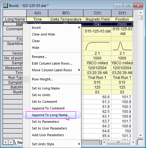
Combine columns in Excel without losing data - 3 quick ways Select both columns you want to merge: click on B1, press Shift + Right Arrrow to select C1, then press Ctrl + Shift + Down Arrow to select all the cells with data in two columns. Copy data to clipboard (press Ctrl + C or Ctrl + Ins, whichever you prefer). Open Notepad: Start-> All Programs -> Accessories -> Notepad . Add Data Labels From Different Column In An Excel Chart A.docx Batch Add All Data Labels From Different Column In An Excel Chart This method will introduce a solution to add all data labels from a different column in an Excel chart at the same time. Please do as follows: 1. Right click the data series in the chart, and selectAdd Data Labels>Add DataLabelsfrom the context menu to add data labels. 2. Column Chart with Category Axis Labels Between Columns Click the menu key (between the right Alt and Ctrl buttons on most Windows keyboards) or hold Shift and click the F10 function key to pop up the context menu. Click Change Series Chart Type, and choose XY Scatter. This adds a set of markers along the bottom of the chart (I used blue circles in the chart below) and it adds secondary X and Y axes. Apply Custom Data Labels to Charted Points - Peltier Tech Select an individual label (two single clicks as shown above, so the label is selected but the cursor is not in the label text), type an equals sign in the formula bar, click on the cell containing the label you want, and press Enter. The formula bar shows the link (=Sheet1!$D$3). Repeat for each of the labels.
Selecting Data in Different Columns for an Excel Chart We need to select columns in the following dataset using CTRL Key. Firstly, select Column B, and holding the CTRL key select Column D. This CTRL key helps to select these two columns at a time. Secondly, go to Insert > select the Insert Column or Bar Chart option marked below. Thirdly, select the 2-D Clustered Column figure. How to Print Labels from Excel - Lifewire Apr 05, 2022 · Select Mailings > Write & Insert Fields > Update Labels . Once you have the Excel spreadsheet and the Word document set up, you can merge the information and print your labels. Click Finish & Merge in the Finish group on the Mailings tab. Click Edit Individual Documents to preview how your printed labels will appear. Select All > OK . Create a multi-level category chart in Excel - ExtendOffice Select the dots, click the Chart Elements button, and then check the Data Labels box. 23. Right click the data labels and select Format Data Labels from the right-clicking menu. 24. In the Format Data Labels pane, please do as follows. 24.1) Check the Value From Cells box; python - Changing inconsistent excel column names into a single name ... I have an excel document with hundreds of sheets that has the same data, except the sheet columns are not uniformly labeled, one column I need in particular has three different column names that vary by sheet. Example Excel Workbook:
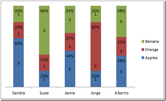
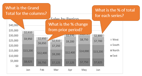
Friday Challenge Answer - Create a Percentage (%) and Value Label within 100% Stacked Chart ...
How can I add data labels from a third column to a scatterplot? Under Labels, click Data Labels, and then in the upper part of the list, click the data label type that you want. Under Labels, click Data Labels, and then in the lower part of the list, click where you want the data label to appear. Depending on the chart type, some options may not be available.
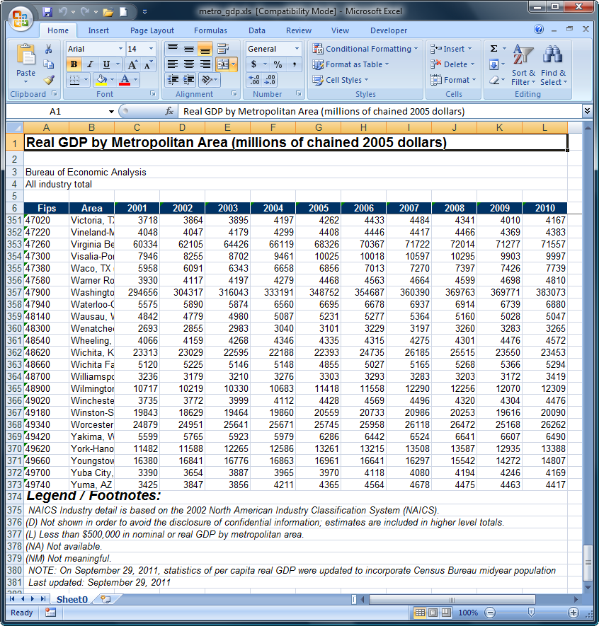
The Stata Blog » Using import excel with real world data
VLOOKUP --> Obtaining data from different columns ... - Excel Help Forum Hello everyone, I would need to solve this basic issue: I am trying to vlookup values from specific columns within an array according to a certain 'label' contained in another column. I have attached a simplified example of my task that is for sure much more straightforward than my above explanation. Many thanks for the help! Cheers, Patrizio
How to add data labels from different column in an Excel chart?
How to Use Cell Values for Excel Chart Labels Select range A1:B6 and click Insert > Insert Column or Bar Chart > Clustered Column. The column chart will appear. We want to add data labels to show the change in value for each product compared to last month. Select the chart, choose the "Chart Elements" option, click the "Data Labels" arrow, and then "More Options."
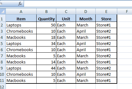
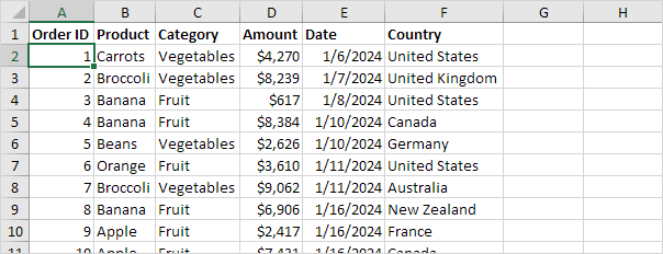
How to Create Pivot Table in Excel
Can I add data labels from an unrelated column to a simple 2 ... I would like to add data labels to the vertical chart representations with values from a third column. I am trying to show how many input/data points were included for each displayed column percentage (height) on the chart. The third column values range from 10-200, with an couple outliers up to 5,500, so a third axis doesn't display the data well.
33 Create Label In Excel - Labels For You
VLOOKUP Hack #4: Column Labels - Excel University This MATCH function would return 2 since the Amount label is in the 2nd table column. So, replacing the 2 in our original formula with the MATCH function would look like this: =VLOOKUP (B5, Table1, MATCH (C4,Table1 [#Headers],0), 0) This technique allows us to reference the column labels instead of the position number. But, Jeff, hang on.
Format Number Options for Chart Data Labels in Excel 2011 for Mac
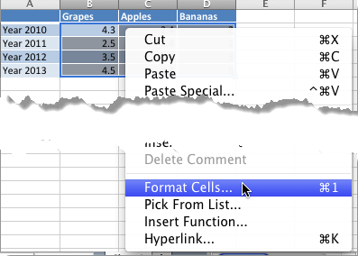
Custom Data Labels with Colors and Symbols in Excel Charts - [How To] Step 4: Select the data in column C and hit Ctrl+1 to invoke format cell dialogue box. From left click custom and have your cursor in the type field and follow these steps: Press and Hold ALT key on the keyboard and on the Numpad hit 3 and 0 keys. Let go the ALT key and you will see that upward arrow is inserted.

30 What Is A Data Label In Excel - Labels Database 2020
How to create Custom Data Labels in Excel Charts Create the chart as usual. Add default data labels. Click on each unwanted label (using slow double click) and delete it. Select each item where you want the custom label one at a time. Press F2 to move focus to the Formula editing box. Type the equal to sign. Now click on the cell which contains the appropriate label.

How to edit the label of a chart in Excel? - Stack Overflow
Move data labels - support.microsoft.com Click any data label once to select all of them, or double-click a specific data label you want to move. Right-click the selection > Chart Elements > Data Labels arrow, and select the placement option you want. Different options are available for different chart types.

Pivot table row labels in separate columns • AuditExcel.co.za
Different Ways to Flip the Data in Excel: Reverse the Data Columns and ... Steps. 1. Type 1 into the 1st and 2 in the 2nd cells. Using your Caesar, double click on the helper column for the autofill of the column with numbers. 2. Cell selection. Select the cells in which you have just entered the numbers and double click the lower right corner of the section. The Excel will autofill the column with serial numbers up ...

Enable or Disable Excel Data Labels at the click of a button - How To - PakAccountants.com
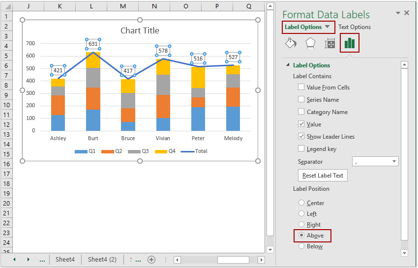
How to add data labels from different column in an Excel chart? Batch add all data labels from different column in an Excel chart. 1. Right click the data series in the chart, and select Add Data Labels > Add Data Labels from the context menu to add data labels. 2. Right click the data series, and select Format Data Labels from the context menu. 3. In the Format ...

How to Show Data in an Intuitive Radar Chart in Your Excel Worksheet - Data Recovery Blog
How to Change Excel Chart Data Labels to Custom Values? You can change data labels and point them to different cells using this little trick. First add data labels to the chart (Layout Ribbon > Data Labels) Define the new data label values in a bunch of cells, like this: Now, click on any data label. This will select "all" data labels. Now click once again.

Enable or Disable Excel Data Labels at the click of a button - How To - PakAccountants.com
Create Dynamic Chart Data Labels with Slicers - Excel Campus You basically need to select a label series, then press the Value from Cells button in the Format Data Labels menu. Then select the range that contains the metrics for that series. Click to Enlarge Repeat this step for each series in the chart. If you are using Excel 2010 or earlier the chart will look like the following when you open the file.
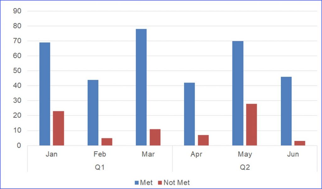
How to Create a Chart with the Axis having Two Categories - ExcelNotes
[SOLVED] Another column as data label? [SOLVED] - Excel Help Forum Make a second series with same values but yr aliases as categories. Plot this new series on a second category axis. Effectively make the new bars completely invisible by selecting the attributes for fill and line to 'none'. Now select for the invisible series the data label and you shd get the desired effect.
Frequency Distribution in Excel - Easy Excel Tutorial

How to sort in Excel Tables
How to add total labels to stacked column chart in Excel?
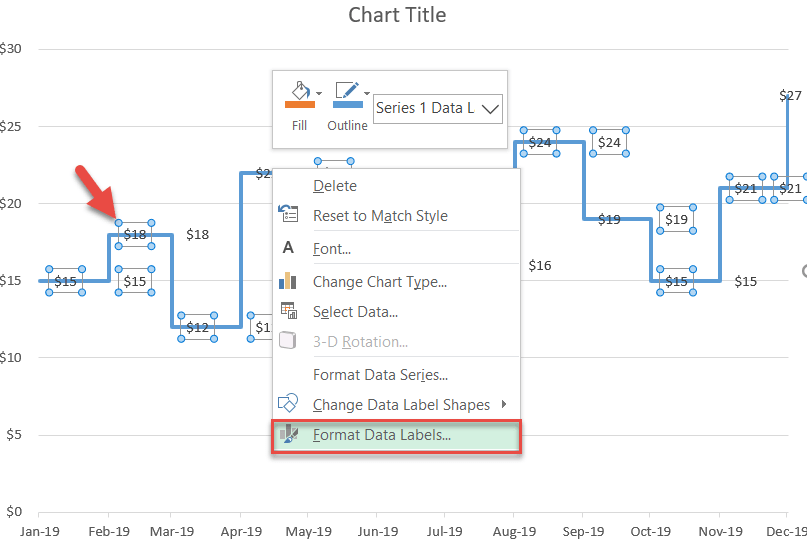
How to Create a Step Chart in Excel - Automate Excel
Label Columns In Excel - Ythoreccio
Post a Comment for "44 excel data labels from different column"