42 how to insert data labels in excel pie chart
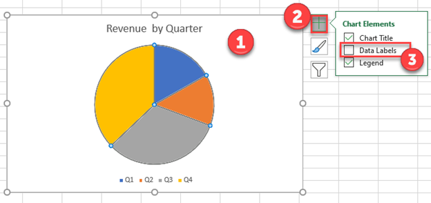
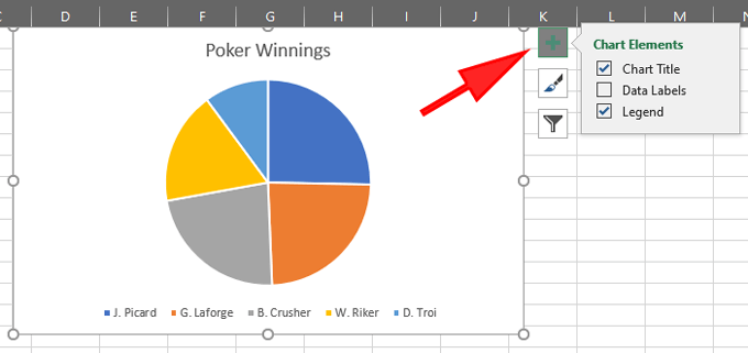
Add or remove data labels in a chart - Microsoft Support Add data labels to a chart · Click the data series or chart. · In the upper right corner, next to the chart, click Add Chart Element · To change the location, ... › examples › pie-chartCreate a Pie Chart in Excel (In Easy Steps) - Excel Easy 6. Create the pie chart (repeat steps 2-3). 7. Click the legend at the bottom and press Delete. 8. Select the pie chart. 9. Click the + button on the right side of the chart and click the check box next to Data Labels. 10. Click the paintbrush icon on the right side of the chart and change the color scheme of the pie chart. Result: 11.
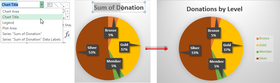
Excel charts: add title, customize chart axis, legend and data labels In Excel 2013 - 365, a chart is already inserted with the default "Chart Title". To change the title text, simply select that box and type your ...
How to insert data labels in excel pie chart
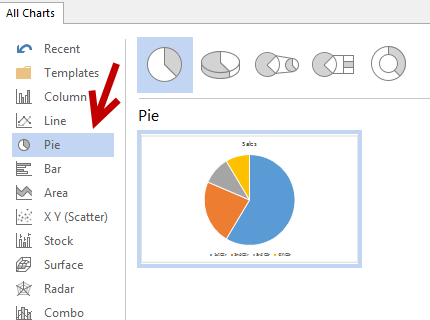
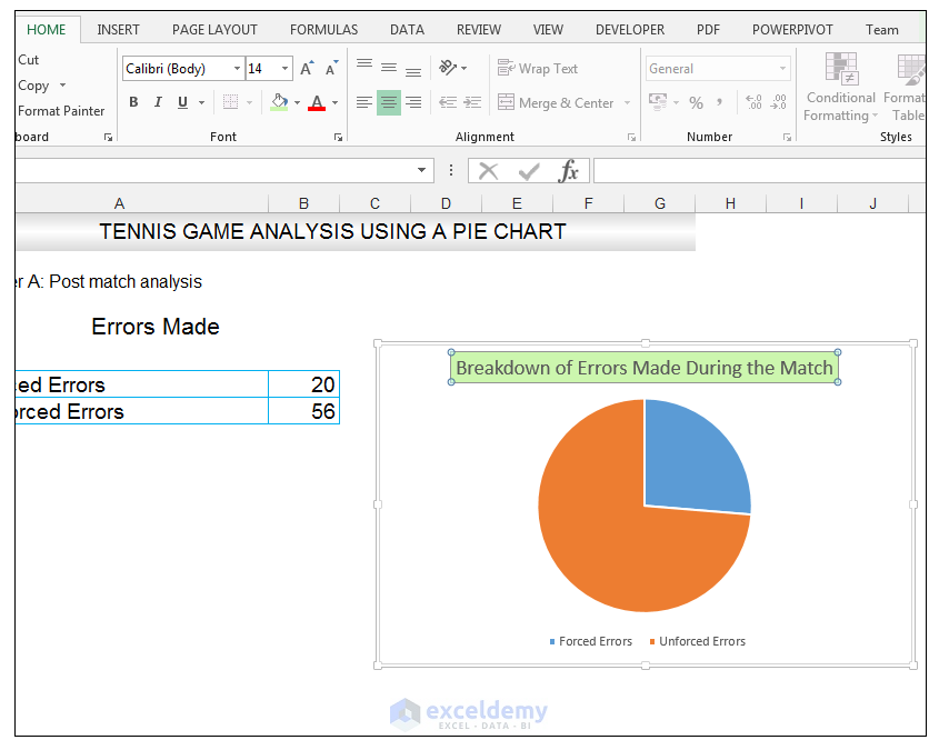
› how-to-create-excel-pie-chartsHow to Make a Pie Chart in Excel & Add Rich Data Labels to ... Sep 08, 2022 · 2) Go to Insert> Charts> click on the drop-down arrow next to Pie Chart and under 2-D Pie, select the Pie Chart, shown below. 3) Chang the chart title to Breakdown of Errors Made During the Match, by clicking on it and typing the new title. › pie-chart-in-excelPie Chart in Excel | How to Create Pie Chart | Step-by-Step ... Step 1: Do not select the data; rather, place a cursor outside the data and insert one PIE CHART. Go to the Insert tab and click on a PIE. Go to the Insert tab and click on a PIE. Step 2: once you click on a 2-D Pie chart, it will insert the blank chart as shown in the below image. trumpexcel.com › pie-chartHow to Make a PIE Chart in Excel (Easy Step-by-Step Guide) Creating a Pie Chart in Excel. To create a Pie chart in Excel, you need to have your data structured as shown below. The description of the pie slices should be in the left column and the data for each slice should be in the right column. Once you have the data in place, below are the steps to create a Pie chart in Excel: Select the entire dataset
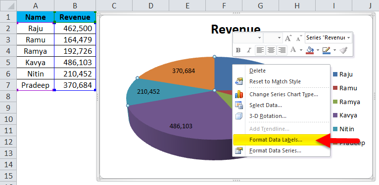
How to insert data labels in excel pie chart. support.microsoft.com › en-us › officePresent data in a chart - support.microsoft.com To see all available chart types, click a chart type, and then click All Chart Types or the More menu item to display the Insert Chart dialog box, click the arrows to scroll through all available chart types and chart subtypes, and then click the ones that you want to use. Change the format of data labels in a chart - Microsoft Support Click the data labels whose border you want to change. Click twice to change the border for just one data label. · Click Fill & Line > Border, and then make the ... How to display leader lines in pie chart in Excel? - ExtendOffice 1. Click at the chart, and right click to select Format Data Labels from context menu. · 2. In the popping Format Data Labels dialog/pane, check Show Leader ... How to insert data labels to a Pie chart in Excel 2013 - YouTube Jun 10, 2013 ... This video will show you the simple steps to insert Data Labels in a pie chart in Microsoft® Excel 2013. Content in this video is provided ...
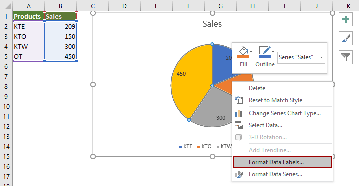
Pie chart in Excel with data labels instead of hard to read legend Oct 22, 2021 ... 00:00 Create Pie Chart in Excel00:13 Remove legend from a chart00:18 Add labels to each slice in a pie chart00:29 Change chart labels to ... How to Label a Pie Chart in Excel (6 Steps) - ItStillWorks Clicking on the data series or a specific data point will open the "Chart Tools" tab. Locate the "Labels" group and click on the "Layout" tab. Click the "Data ... › documents › excelHow to create pie of pie or bar of pie chart in Excel? And then click Insert > Pie > Pie of Pie or Bar of Pie, see screenshot: 3. And you will get the following chart: 4. Then you can add the data labels for the data points of the chart, please select the pie chart and right click, then choose Add Data Labels from the context menu and the data labels are appeared in the chart. See screenshots: Adding Data Labels to Your Chart - Excel ribbon tips Aug 27, 2022 ... Activate the chart by clicking on it, if necessary. · Make sure the Layout tab of the ribbon is displayed. · Click the Data Labels tool. Excel ...
› create-a-pie-chart-in-excel-3123565How to Create and Format a Pie Chart in Excel - Lifewire Jan 23, 2021 · Add Data Labels to the Pie Chart . There are many different parts to a chart in Excel, such as the plot area that contains the pie chart representing the selected data series, the legend, and the chart title and labels. All these parts are separate objects, and each can be formatted separately. trumpexcel.com › pie-chartHow to Make a PIE Chart in Excel (Easy Step-by-Step Guide) Creating a Pie Chart in Excel. To create a Pie chart in Excel, you need to have your data structured as shown below. The description of the pie slices should be in the left column and the data for each slice should be in the right column. Once you have the data in place, below are the steps to create a Pie chart in Excel: Select the entire dataset › pie-chart-in-excelPie Chart in Excel | How to Create Pie Chart | Step-by-Step ... Step 1: Do not select the data; rather, place a cursor outside the data and insert one PIE CHART. Go to the Insert tab and click on a PIE. Go to the Insert tab and click on a PIE. Step 2: once you click on a 2-D Pie chart, it will insert the blank chart as shown in the below image. › how-to-create-excel-pie-chartsHow to Make a Pie Chart in Excel & Add Rich Data Labels to ... Sep 08, 2022 · 2) Go to Insert> Charts> click on the drop-down arrow next to Pie Chart and under 2-D Pie, select the Pie Chart, shown below. 3) Chang the chart title to Breakdown of Errors Made During the Match, by clicking on it and typing the new title.
Excel Doughnut chart with leader lines – teylyn
How to show percentage in pie chart in Excel?

Change the format of data labels in a chart

How to Make a Pie Chart in Excel
Help Online - Quick Help - FAQ-1019 How to customize the font ...
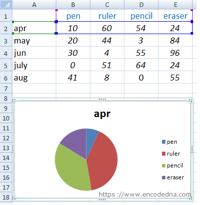
How to Create a Pie Chart in Excel using Worksheet Data

Optimally positioning pie chart data labels in Excel with VBA ...

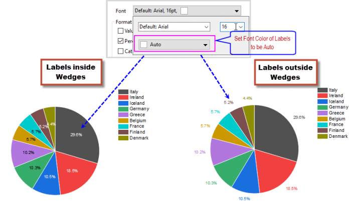
How to Make Pie Chart with Labels both Inside and Outside ...

Add or remove data labels in a chart

How to Make an Excel Pie Chart
How to Add Data Callout Labels to Charts in Excel in C#

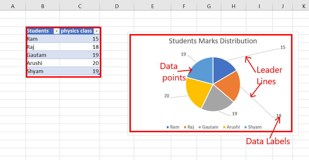
How-to Add Label Leader Lines to an Excel Pie Chart - Excel ...
Create Outstanding Pie Charts in Excel | Pryor Learning

Presenting Data with Charts
Office: Display Data Labels in a Pie Chart
How to Make a Pie Chart in Excel & Add Rich Data Labels to ...

Chart Data Labels in PowerPoint 2013 for Windows

Pie Chart – Excel Tutorials
Plotting Charts | Aprende con Alf
How to Add Leader Lines in Excel? - GeeksforGeeks

how to add data labels into Excel graphs — storytelling with data
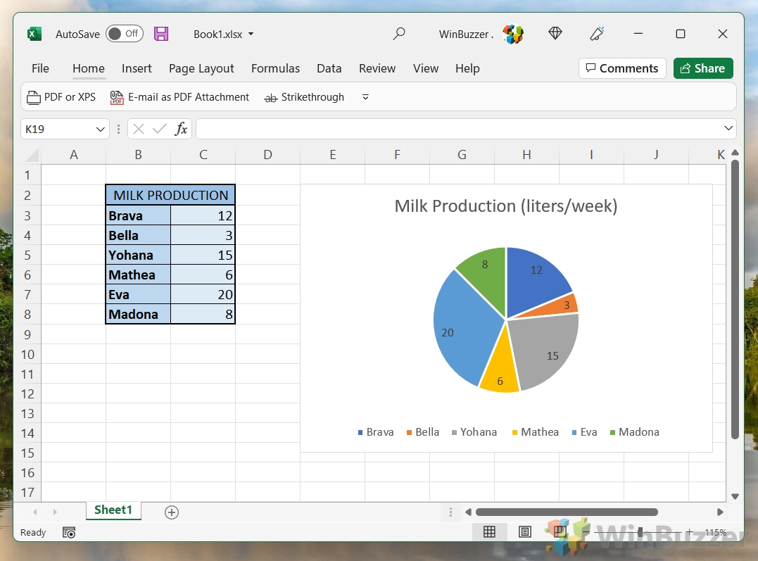
How to Make a Pie Chart in Excel - WinBuzzer

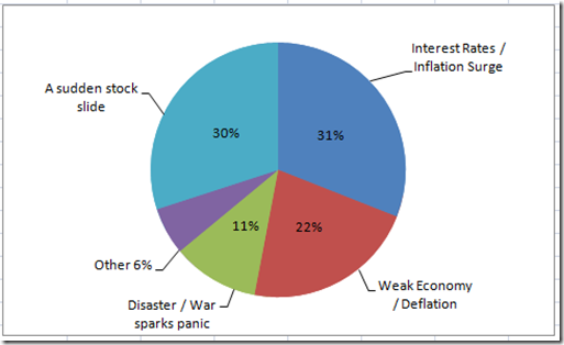
How to Show Percentage in Pie Chart in Excel? - GeeksforGeeks
Pie Chart - Show Percentage - Excel & Google Sheets ...
Pie Chart in Excel | How to Create Pie Chart | Step-by-Step ...

Inserting Data Label in the Color Legend of a pie chart ...

How to Data Labels in a Pie chart in Excel 2010
How-to Make a WSJ Excel Pie Chart with Labels Both Inside and ...

How to Make Pie Chart with Labels both Inside and Outside ...

Excel Doughnut chart with leader lines – teylyn
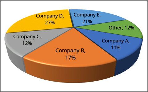
Excel 3-D Pie charts - Microsoft Excel 365

How to Create a Pie Chart in Excel | Smartsheet

How to Add Data Labels to an Excel 2010 Chart - dummies
How to Make a Pie Chart in Excel

Change the format of data labels in a chart

Creating Pie Chart and Adding/Formatting Data Labels (Excel)

Add data labels and callouts to charts in Excel 365 ...

Change color of data label placed, using the 'best fit ...

Adding Data Labels to Your Chart (Microsoft Excel)
5 New Charts to Visually Display Data in Excel 2019 - dummies

How to make a pie chart in Excel
Pie Chart in Excel | How to Create Pie Chart | Step-by-Step ...
Post a Comment for "42 how to insert data labels in excel pie chart"