39 excel pivot table conditional formatting row labels

Conditional Formatting on Pivot Table row labels Re: Conditional Formatting on Pivot Table row labels Hi Dilip, The date is a "date" and not a text. What I mean is each cell in A should be compared with the 3 dates in E and should do the conditional formatting (excel icon sets) accordingly. If you see the cell A in srcFromWorkSheet you know what I mean. Please let me know if you have any queries. Excel tutorial: Conditional formatting formula in a table This allows the formula to highlight an entire row. Now I'll use this formula to create the conditional formatting rule. As you can see, the rule correctly highlights employees in group A. Even though we can't use structured references, we still get some benefit from using a table, because Excel will keep track of the table range.

Excel VBA: Conditional Format of Pivot Table based on Column Label ... myPivotSourceName = myPivotField.Name. Then rather than referencing the data field with the pivot field object, I referenced the DataRange with the string: myPivotTable.PivotFields (myPivotSourceName).DataRange.Select. Works perfectly and is completely portable for any pivottable on any sheet with any fields. excel vba.

Excel pivot table conditional formatting row labels

Conditional Formatting in Pivot Table - WallStreetMojo Currently, a pivot table is blank. Next, we need to bring in the values. Then, drag down the "Date" in the "Rows" Label, "Name" in the "Column," and "Sales" in "Values." As a result, the pivot table will look like the one below. To apply conditional formatting in the pivot table, first, we must select the column to format. Pivot Table Conditional Formatting - Contextures Excel Tips We'll adjust the formatting range, to fix that problem. Select any cell in the pivot table. On the Ribbon's Home tab, click Conditional Formatting, then click Manage Rules. In the list of rules, select the Data Bar rule, which applies to cells B3:B8. Click Edit Rule, to open the Edit Formatting Rule window. How to apply conditional formatting to Pivot Tables - SpreadsheetWeb Go to HOME > Conditional Formatting > New Rule to add a new formatting rule, or select from predefined options. If you select the latter, you will need to configure the rule regardless. The New (or Edit) Formatting Rule window contains options specific to Pivot Tables. You can choose the location where you want to apply your conditional ...

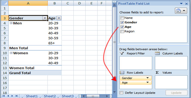
Excel pivot table conditional formatting row labels. How to Create Pivot Tables in Excel (In Easy Steps) Insert a Pivot Table. To insert a pivot table, execute the following steps. 1. Click any single cell inside the data set. 2. On the Insert tab, in the Tables group, click PivotTable. The following dialog box appears. Excel automatically selects the data for you. The default location for a new pivot table is New Worksheet. 3. Click OK. Drag fields How to Apply Conditional Formatting to Pivot Tables - Excel … 13.12.2018 · Bottom Line: Learn how to apply conditional formatting to pivot tables so that the formats are dynamically reapplied as the pivot table is changed, filtered, or updated. Skill Level: Intermediate Download the Excel File. Here's the file that I use in the video. You can use it to practice adding, deleting, and changing conditional formatting on a variety of pivot table … Pivot Table Conditional Formatting Weirdness: Range Changing Itself : excel This table is turned into a small summary table, a pivot table, and a pivot chart. Using the wonderful resources of stack overflow and Google, I finally got the next step. I now have a script in PowerShell that opens the workbook, runs the query, updates, the pivots, saves and closes, then emails this to the relevant managers. Apply conditional formatting for each row in Excel - ExtendOffice Apply conditional formatting for each row in Excel As we know, the Conditional Formatting will create a rule to determine which cells will be format. Sometimes, you may want to apply the conditional formatting for per row as below screenshot shown. Except repeatedly setting the same rules for per row, there are some tricks on solving this job.

Pivot Table Conditional Formatting with VBA - Peltier Tech Note that refreshing the pivot tables changes values but does not automatically reformat the tables. You have to manually rerun the VBA routines, or capture the PivotTableUpdate event: Private Sub Worksheet_PivotTableUpdate (ByVal Target As PivotTable) Select Case Target.Name Case "PivotTable1" FormatPT1 Case "PivotTable2" FormatPT2 End Select ... Format Pivot Table Labels Based on Date Range Select all the dates in the Row Labels that you want to format. On the Ribbon, click the Home tab, and then in the Styles group, click Conditional Formatting. In the list of conditional formatting options, click Highlight Cells Rules, and then click A Date Occurring. How to Group Numbers in Pivot Table in Excel - Trump Excel Sometimes, numbers are stored as text in Excel. In such case, you need to convert these text to numbers before grouping it in Pivot Table. You May Also Like the Following Pivot Table Tutorials: How to Group Dates in Pivot Table in Excel. How to Create a Pivot Table in Excel. Preparing Source Data For Pivot Table. How to Refresh Pivot Table in ... How to Apply Conditional Formatting to Rows Based on Cell Value - Excel ... On the Home tab of the Ribbon, select the Conditional Formatting drop-down and click on Manage Rules…. That will bring up the Conditional Formatting Rules Manager window. Click on New Rule. This will open the New Formatting Rule window. Under Select a Rule Type, choose Use a formula to determine which cells to format.

Pivot Table: Pivot table conditional formatting | Exceljet Select any cell in the data you wish to format and then choose "New rule" from the conditional formatting menu on the Home tab of the ribbon. At the top of the window, you will see setting for which cells to apply conditional formatting to. For the example shown, we want: "All cells showing sum of "sales values" for name and "date" How to Filter Data in Pivot Table with Examples - EDUCBA How to Filter a Pivot Table in Excel? Introduction to Pivot Table Filter. A Pivot Table filter is something that we get when we create a pivot table by default. First, create a table using a Pivot Table; we can see the first field, which is either a Row or Column, will have one filter. Click on the drop-down arrow or press the ALT + Down ... Apply Conditional Formatting | Excel Pivot Table Tutorial Go to Home Tab → Styles → Conditional Formatting → New Rule. From rule to, select the third option. And, from "select a rule" type select "Format only top or bottom" ranked values. In edit rule description, enter 1 in the input box and from the drop-down menu select "each Column Group". Apply formatting you want. Click OK. conditional formatting per row on pivot - Microsoft Tech Community conditional formatting per row on pivot. I would like to format each row of a pivot table separately (as in the picture shown below), but I cannot paste the formatting. I've got many rows, and they could change (just like the columns) Is there a way to automate this, or I have to select row by row and apply the formatting?

How to remove bold font of pivot table in Excel?

How to remove bold font of pivot table in Excel? - ExtendOffice The normal Bold feature can’t help us to un-bold the row labels in pivot table, but we can apply the powerful function – Conditional Formatting to solve this problem. Please do as follows: 1. Select the bold font row you want to un-bold in the pivot table, or you can press Ctrl key to select multiple bold font rows as your need. See screenshot:

Lesson 54: Pivot Table Row Labels - Swotster

101 Advanced Pivot Table Tips And Tricks You Need To Know Apr 25, 2022 · Without a table your range reference will look something like above. In this example, if we were to add data past Row 51 or Column I our pivot table would not include it in the results. To create and name your table. Select your data. Go to the Insert tab and press the Table button in the Tables section, or use the keyboard shortcut Ctrl + T.

vba - Pivot Table with Conditional Formatting: Where did my indents go? - Stack Overflow

Design the layout and format of a PivotTable To change the layout of a PivotTable, you can change the PivotTable form and the way that fields, columns, rows, subtotals, empty cells and lines are displayed. To change the format of the PivotTable, you can apply a predefined style, banded rows, and conditional formatting. Windows Web Mac Changing the layout form of a PivotTable

How to Insert a Blank Row in Excel Pivot Table | MyExcelOnline

Excel Conditional Formatting in Pivot Table - EDUCBA Click on any cell in the pivot table > Go to the HOME tab > Click on Conditional Formatting option under Styles option > Click on Manage Rules option. It will open a Rules Manager dialog box. Click on the Edit Rule tab, as shown in the below screenshot. It will open the Editing Rule formatting window. Refer to the below screenshot.

√ダウンロード change table name excel 365 255677-Office 365 excel change table name

The Pivot table tools ribbon in Excel These two tabs allow you to perform pivot table customization. This is the Pivot table ribbon in Excel. Create pivot table fields , charts and sets. Here is an important thing to wonder for the pivot table ribbon in excel is as soon as you switch the selected cell to non pivot table cell. The pivot table ribbon disappears. So it means Excel ...

How to Create a MS Excel Pivot Table – An Introduction | SIMPLE TAX INDIA

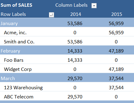
How To Compare Multiple Lists of Names with a Pivot Table 08.07.2014 · Column E of the Pivot Table contains the Grand Total (sum of columns B:D). People that volunteered all three years will have a “3” in column E. We should sort the pivot table so all the people with a “3” in column E appear at the top of the list. This will make it …

Excel Tutorial: Pivot Table and Chart in Financial Modelling

Highlight Cell Rules based on date labels | MyExcelOnline This is our current Pivot Table setup. We want to highlight all of the dates of the current month (July 2021) in our Row Labels. Example 1: STEP 1: Highlight all the date labels by clicking above the cell. STEP 2: Go to Home > Conditional Formatting > Highlight Cells Rules > A Date Occuring. STEP 3: Select This Month and select OK.

Excel - Beyond the Basics Part Two: Using Conditional Formatting in a Pivot Table - United ...

Pivot Table Conditional Formatting - Microsoft Tech Community Hi all :) I have an issue conditionally formatting a Pivot Table. I have my row hierarchy set up as Region, Area, Store, Consultant. My rows are expanded out only to a Store Level. I need the Store Name to be highlighted red if the value in the first column is <1. I have applied conditional fo...

Share :