39 how to add two data labels in excel pie chart

How to Customize Your Excel Pivot Chart Data Labels - dummies To add data labels, just select the command that corresponds to the location you want. To remove the labels, select the None command. If you want to specify what Excel should use for the data label, choose the More Data Labels Options command from the Data Labels menu. Excel displays the Format Data Labels pane. › 2015/11/12 › make-pie-chart-excelHow to make a pie chart in Excel - Ablebits Nov 12, 2015 · Adding data labels to a pie chart; Showing data categories on the labels; Excel pie chart percentage and value; Adding data labels to Excel pie charts. In this pie chart example, we are going to add labels to all data points. To do this, click the Chart Elements button in the upper-right corner of your pie graph, and select the Data Labels ...

› pie-chart-examplesPie Chart Examples | Types of Pie Charts in Excel ... - EDUCBA Now our task is to add the Data series to the PIE chart divisions. Click on the PIE chart so that the chart will get a highlight, as shown below. Right-click and choose the “Add Data Labels “option for additional drop-down options.

How to add two data labels in excel pie chart

Possible to add second data label to pie chart? - Excel Help Forum Re: Possible to add second data label to pie chart? Create the composite label in a worksheet column by concatenating the data in other cells and the nextline character, CHR (10). Now, use this composite label column as the source for Rob Bovey's add-in. -- Regards, Tushar Mehta Excel, PowerPoint, and VBA add-ins, tutorials › charts › add-data-pointAdd Data Points to Existing Chart – Excel & Google Sheets Start with your Graph. Similar to Excel, create a line graph based on the first two columns (Months & Items Sold) Right click on graph; Select Data Range; 3. Select Add Series. 4. Pivot Chart Data Label Help Needed - Microsoft Community Open the Excel file with Pivot Chart and enabled with Data Labels> Click on the Labels displayed in the Chart> Right-click> Click Format Data Labels> Label Options> Number> In the Category, select the format as per your requirement. Here is the reference article: Change the format of data labels in a chart.

How to add two data labels in excel pie chart. How To Show Two Sets of Data on One Graph in Excel Below are steps you can use to help add two sets of data to a graph in Excel: 1. Enter data in the Excel spreadsheet you want on the graph. To create a graph with data on it in Excel, the data has to be represented in the spreadsheet. For multiple variables that you want to see plotted on the same graph, entering the values into different ... How to Create and Format a Pie Chart in Excel - Lifewire To add data labels to a pie chart: Select the plot area of the pie chart. Right-click the chart. Select Add Data Labels . Select Add Data Labels. In this example, the sales for each cookie is added to the slices of the pie chart. Change Colors Add data labels and callouts to charts in Excel 365 - EasyTweaks.com Step #1: After generating the chart in Excel, right-click anywhere within the chart and select Add labels . Note that you can also select the very handy option of Adding data Callouts. Step #2: When you select the "Add Labels" option, all the different portions of the chart will automatically take on the corresponding values in the table ... How to add data labels from different column in an Excel chart? Right click the data series in the chart, and select Add Data Labels > Add Data Labels from the context menu to add data labels. 2. Click any data label to select all data labels, and then click the specified data label to select it only in the chart. 3.

Adding data labels to a pie chart - Excel General - OzGrid Re: Adding data labels to a pie chart. Thanks again, norie. Really appreciate the help. I tried recording a macro while doing it manually (before my first post). But it didn't record anything about labels, much less making them bold. › charts › axis-labelsHow to add Axis Labels (X & Y) in Excel & Google Sheets How to Add Axis Labels (X&Y) in Excel. Graphs and charts in Excel are a great way to visualize a dataset in a way that is easy to understand. The user should be able to understand every aspect about what the visualization is trying to show right away. As a result, including labels to the X and Y axis is essential so that the user can see what ... › ms-excel-pie-chartHow to Make a Pie Chart in Excel (Only Guide You Need) Sep 13, 2021 · How to Insert Data into a Pie Chart in Excel. The first condition of making a pie chart in Excel is to make a table of data. In this example, we will see the process of inserting data from a table to make a pie chart. Here we will be analyzing the attendance list of 5 months of some students in a course. The table s given below. How to Create Pie Charts in Excel (In Easy Steps) Click the + button on the right side of the chart and click the check box next to Data Labels. 10. Click the paintbrush icon on the right side of the chart and change the color scheme of the pie chart. Result: 11. Right click the pie chart and click Format Data Labels. 12. Check Category Name, uncheck Value, check Percentage and click Center.

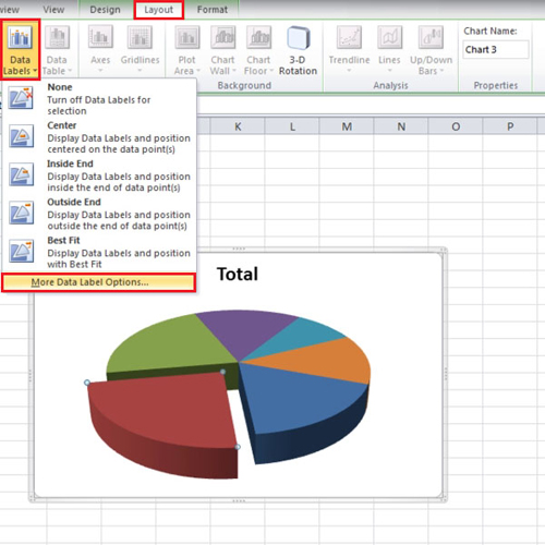
How to Add Data Labels to an Excel 2010 Chart - dummies Use the following steps to add data labels to series in a chart: Click anywhere on the chart that you want to modify. On the Chart Tools Layout tab, click the Data Labels button in the Labels group. None: The default choice; it means you don't want to display data labels. Center to position the data labels in the middle of each data point. Pie Chart in Excel - Inserting, Formatting, Filters, Data Labels To add Data Labels, Click on the + icon on the top right corner of the chart and mark the data label checkbox. You can also unmark the legends as we will add legend keys in the data labels. We can also format these data labels to show both percentage contribution and legend:- Right click on the Data Labels on the chart. How to Create Multi-Category Charts in Excel? - GeeksforGeeks Step 1: Insert the data into the cells in Excel. Now select all the data by dragging and then go to "Insert" and select "Insert Column or Bar Chart". A pop-down menu having 2-D and 3-D bars will occur and select "vertical bar" from it. Select the cell -> Insert -> Chart Groups -> 2-D Column. How to Combine or Group Pie Charts in Microsoft Excel Click on the first chart and then hold the Ctrl key as you click on each of the other charts to select them all. Click Format > Group > Group. All pie charts are now combined as one figure. They will move and resize as one image. Choose Different Charts to View your Data

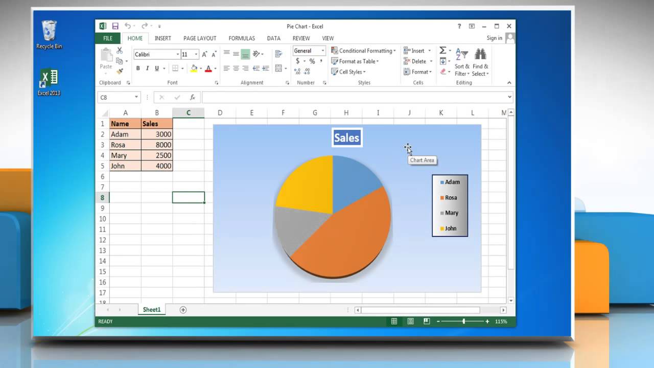
How to insert data labels in a Pie chart in Excel 2013 - YouTube

How To Create A Pie Chart In Excel - PieProNation.com With everything we need in place, its time to create a pie chart using the pivot table you just built. Select any cell in your pivot table . Navigate to the Insert tab. Hit the Insert Pie or Doughnut Chart button. Under 2-D Pie, click Pie. Once you do that, Excel will automatically plot a pie graph using your pivot table.

How can someone create a pie chart with 2 variables in MS Excel? - Quora

excel - Positioning data labels in pie chart - Stack Overflow Sub tester () Dim se As Series Set se = Totalt.ChartObjects ("Inosa gule").Chart.SeriesCollection ("Grøn pil") se.ApplyDataLabels With se.DataLabels .NumberFormat = "0,0 %" With .Format.Fill .ForeColor.RGB = RGB (255, 255, 255) .Transparency = 0.15 End With .Position = xlLabelPositionCenter End With End Sub

How to Make a Pie Chart in Microsoft Excel 2010

Creating Pie Chart and Adding/Formatting Data Labels (Excel) Creating Pie Chart and Adding/Formatting Data Labels (Excel) Creating Pie Chart and Adding/Formatting Data Labels (Excel)

How to Create and modify a pie chart in Excel | HowTech

Excel charts: add title, customize chart axis, legend and data labels ... Click anywhere within your Excel chart, then click the Chart Elements button and check the Axis Titles box. If you want to display the title only for one axis, either horizontal or vertical, click the arrow next to Axis Titles and clear one of the boxes: Click the axis title box on the chart, and type the text.

How to Make a Pie Chart in Excel & Add Rich Data Labels to The Chart!

How To Construct a Waterfall Chart - bestmacapp.com To create your waterfall chart, follow these steps: Create a new Excel worksheet and enter headings in row 1: "Label," "Type," and "Amount.". In cell A2, enter "Total Income.". In cell B2, enter "Total Expenses.". In cell C2, enter "Net amount of income.". Select cells A2 through C2 and insert a waterfall chart type by ...

Excel Charting Dos and Don'ts - Peltier Tech Blog

Create two data labels in pie chart? - MrExcel Message Board You have already figured out how to add an image that fills the sector of the pie chart but as far as I know you cannot add an icon or image over the actual pie chart sector, in such a way that it adjusts with the values. If you add it as a static image next to the legend, at least the legend does not move when the values change. Paul.

How to Make a Pie Chart in Excel & Add Rich Data Labels to The Chart!

Pie of Pie Chart in Excel - Inserting, Customizing, Formatting To add the data labels:- Select the chart and click on + icon at the top right corner of chart. Mark the check box containing data labels. Formatting Data Labels Consequently, this is going to insert default data labels on the chart.

How to Make a Pie Chart in Excel & Add Rich Data Labels to The Chart!

How to add or move data labels in Excel chart? - ExtendOffice To add or move data labels in a chart, you can do as below steps: In Excel 2013 or 2016. 1. Click the chart to show the Chart Elements button . 2. Then click the Chart Elements, and check Data Labels, then you can click the arrow to choose an option about the data labels in the sub menu. See screenshot:

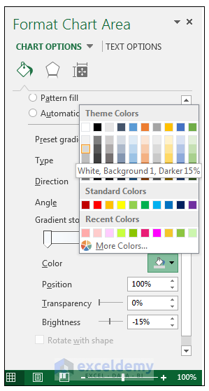
Change color of data label placed, using the 'best fit' option, outside a pie chart - Excel 2010 ...

Edit titles or data labels in a chart - support.microsoft.com On a chart, click one time or two times on the data label that you want to link to a corresponding worksheet cell. The first click selects the data labels for the whole data series, and the second click selects the individual data label. Right-click the data label, and then click Format Data Label or Format Data Labels.

31 Excel Chart Label Axis - Label Design Ideas 2020

How to make a pie chart with two sets of data in Excel - Quora Answer: A pie chart isn't meant to show two sets of data. The pie is 100% of the data and the slices are portions representing what part of the whole each category represents. What are you trying to convey with two datasets? Is it possible you want to make two pie charts side-by-side so people ca...

Pie charts duel to their death: Create slope graphs as an alternative in Tableau in five steps

How to Create a Double Doughnut Chart in Excel - Statology Step 3: Add a layer to create a double doughnut chart. Right click on the doughnut chart and click Select Data. In the new window that pops up, click Add to add a new data series. For Series values, type in the range of values fpr Quarter 2 revenue: Click OK.

How to Make a Pie Chart in Excel & Add Rich Data Labels to The Chart!

› data-series-data-points-dataUnderstanding Excel Chart Data Series, Data Points, and Data ... Sep 19, 2020 · Add Emphasis With a Combo Chart . Another option for emphasizing different types of information in a chart is to display two or more chart types in a single chart, such as a column chart and a line graph. You could use this approach when the graphed values vary widely or when graphing different types of data.

How to Make a Pie Chart in Excel & Add Rich Data Labels to The Chart!

Pie Chart in Excel | How to Create Pie Chart - EDUCBA Step 1: Select the data to go to Insert, click on PIE, and select 3-D pie chart. Step 2: Now, it instantly creates the 3-D pie chart for you. Step 3: Right-click on the pie and select Add Data Labels. This will add all the values we are showing on the slices of the pie.

Share :