38 how to show labels in excel chart
How to show percentage in pie chart in Excel? - ExtendOffice Show percentage in pie chart in Excel. Please do as follows to create a pie chart and show percentage in the pie slices. 1. Select the data you will create a pie chart based on, click Insert > Insert Pie or Doughnut Chart > Pie. See screenshot: 2. Then a pie chart is created. Right click the pie chart and select Add Data Labels from the context ... How to wrap X axis labels in a chart in Excel? - ExtendOffice When the chart area is not wide enough to show it's X axis labels in Excel, all the axis labels will be rotated and slanted in Excel. Some users may think of wrapping the axis labels and letting them show in more than one line. Actually, there are a couple of tricks to warp X axis labels in a chart in Excel. Wrap X axis labels with adding hard ...
How to: Display and Format Data Labels - DevExpress To display value labels, set the DataLabelBase.ShowValue property of the DataLabelOptions object to true. Series name. Series labels identify data series to which the data points in the chart belong. Most series include multiple data points, so the same name will be repeated for all data points in the series, which is probably overkill.
How to show labels in excel chart
How to Add Total Data Labels to the Excel Stacked Bar Chart 03/04/2013 · For stacked bar charts, Excel 2010 allows you to add data labels only to the individual components of the stacked bar chart. The basic chart function does not allow you to add a total data label that accounts for the sum of the individual components. Fortunately, creating these labels manually is a fairly simply process. excel - How to getting text labels to show up in scatter chart - Stack ... How to getting text labels to show up in scatter chart. I want text labels for my scatter plot that is connected with points in the graph. my data is like this. The chart removes the labels and places numbers. How do I get the text labels back? Text Labels on a Horizontal Bar Chart in Excel - Peltier Tech 21/12/2010 · In this tutorial I’ll show how to use a combination bar-column chart, in which the bars show the survey results and the columns provide the text labels for the horizontal axis. The steps are essentially the same in Excel 2007 and in Excel 2003. I’ll show the charts from Excel 2007, and the different dialogs for both where applicable.
How to show labels in excel chart. › how-to-show-percentage-inHow to Show Percentage in Pie Chart in Excel? - GeeksforGeeks Jun 29, 2021 · It can be observed that the pie chart contains the value in the labels but our aim is to show the data labels in terms of percentage. Show percentage in a pie chart: The steps are as follows : Select the pie chart. Right-click on it. A pop-down menu will appear. Click on the Format Data Labels option. The Format Data Labels dialog box will appear. › documents › excelHow to show percentage in pie chart in Excel? - ExtendOffice Show percentage in pie chart in Excel. Please do as follows to create a pie chart and show percentage in the pie slices. 1. Select the data you will create a pie chart based on, click Insert > Insert Pie or Doughnut Chart > Pie. See screenshot: 2. Then a pie chart is created. Right click the pie chart and select Add Data Labels from the context ... How to Add Axis Titles in a Microsoft Excel Chart Select your chart and then head to the Chart Design tab that displays. Click the Add Chart Element drop-down arrow and move your cursor to Axis Titles. In the pop-out menu, select "Primary Horizontal," "Primary Vertical," or both. If you're using Excel on Windows, you can also use the Chart Elements icon on the right of the chart. Excel Chart Vertical Axis Text Labels • My Online Training Hub Now comes the Sneaky Bar Chart; we know that a bar chart has text labels on the vertical axis like this: ... Layout Tab > Axes > Secondary Vertical Axis > Show default axis. Excel 2013: Chart Tools: Design Tab > Add Chart Element > Axes > Secondary Vertical. Now your chart should look something like this with an axis on every side: Let’s cull some of those axes and format …
How to Find, Highlight, and Label a Data Point in Excel Scatter Plot? By default, the data labels are the y-coordinates. Step 3: Right-click on any of the data labels. A drop-down appears. Click on the Format Data Labels… option. Step 4: Format Data Labels dialogue box appears. Under the Label Options, check the box Value from Cells . Step 5: Data Label Range dialogue-box appears. › 509290 › how-to-use-cell-valuesHow to Use Cell Values for Excel Chart Labels Mar 12, 2020 · Select the chart, choose the “Chart Elements” option, click the “Data Labels” arrow, and then “More Options.” Uncheck the “Value” box and check the “Value From Cells” box. Select cells C2:C6 to use for the data label range and then click the “OK” button. How to Use Cell Values for Excel Chart Labels 12/03/2020 · If these cell values change, then the chart labels will automatically update. Link a Chart Title to a Cell Value. In addition to the data labels, we want to link the chart title to a cell value to get something more creative and dynamic. We will begin by creating a useful chart title in a cell. We want to show the total sales in the chart title. How to Use Excel Pivot Table Label Filters You can use a similar technique to hide most of the items in the Row Labels or Column Labels. Select the pivot table items that you want to keep visible Right-click on one of the selected items In the pop-up menu, click Filter, then click Keep Only Selected Items. All but the selected items are immediately hidden in the pivot table.
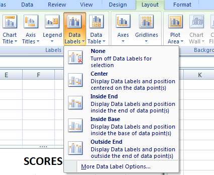
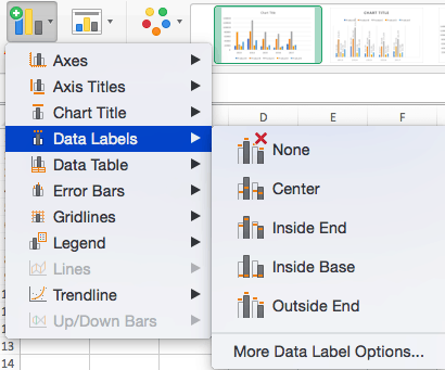
How to avoid data label in excel line chart overlap ... - Stack Overflow I have 2 series of values plotted on the same line chart in Excel (see above). I want to show the data label for both lines on the chart. However, it seems like the data labels will overlap with either the green dot/red dot/line. If I adjust the position of the data labels, it will only work for this 2 series of values. Excel Chart not showing SOME X-axis labels - Super User 05/04/2017 · I was having a similar problem and it was only due to what excel can fit in the chart. Click the chart, and then drag one of the sizing handles to enlarge the chart. By default, the fonts in the chart scale proportionally as you resize the chart. Once you make your chart big enough, your labels should show. 5 New Charts to Visually Display Data in Excel 2019 - dummies To add data labels to the chart, choose Chart Tools Design → Add Chart Element → Data Labels → Show. Pouring Out Data with a Funnel Chart Let's look at one more new chart type: the funnel chart. A funnel chart shows each data point as a horizontal bar, with longer bars for greater values. The bars are all centered and stacked vertically. Pivot Chart Data Label Formatting Question - Microsoft Tech Community Hi, I have a pivot chart. I format the data labels, for example make the text larger or turn it. Every time I refresh the data the data label formatting reverts to the default. I have gone to the Pivot Chart options and made sure the Preserve cell formatting option is checked. How to I get around...
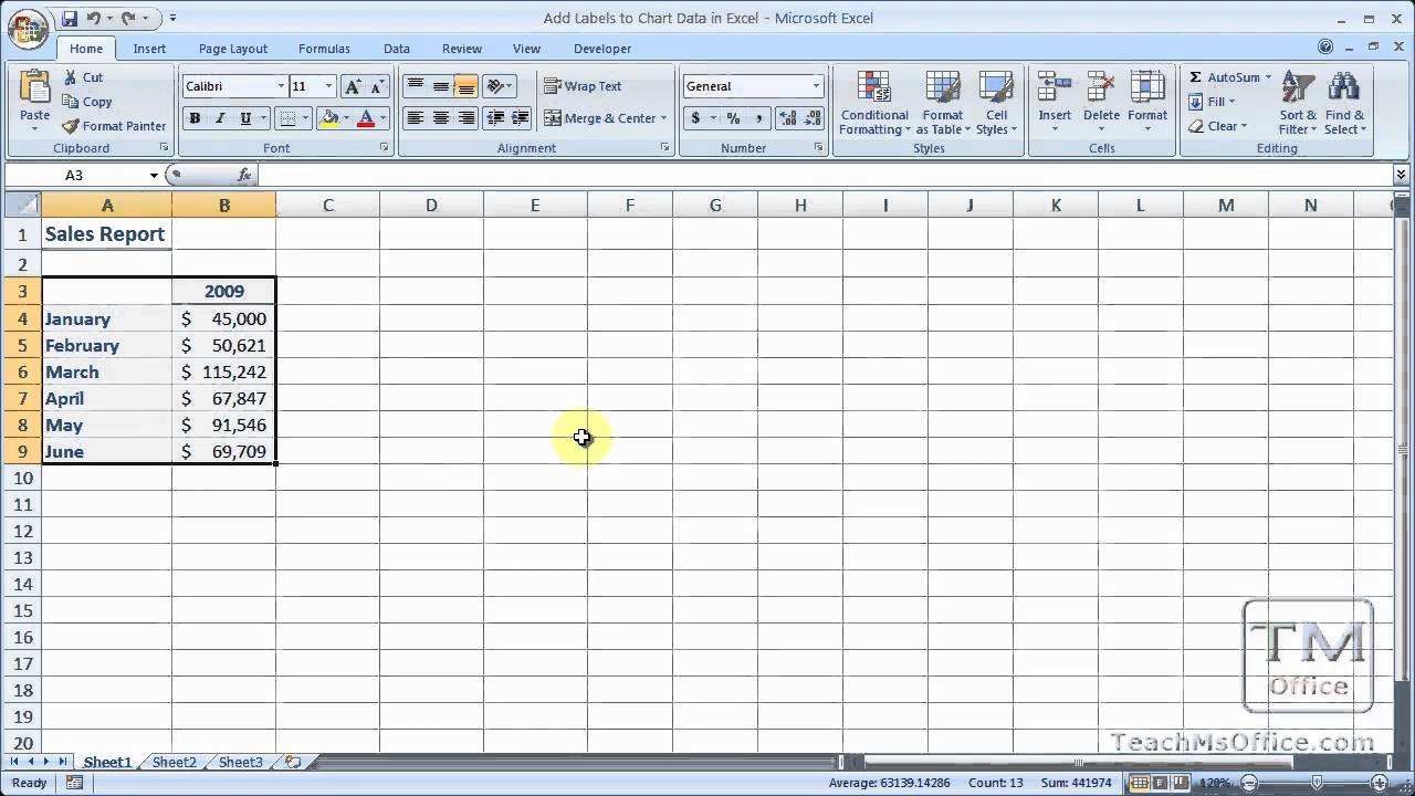
Add Labels to Chart Data in Excel - YouTube
Excel Map Chart not showing DATA LABELS for all INDIAN PROVINCES It seems really inconsistent and I would appreciate Micrsoft looking into this. In this following example, this time with India, I'm trying to get my data label (Provinces and data %'s) to appear in white on the map chart, however, they are refusing to appear even though I clicked on all the right areas for them to do so.
Quickly Create An Actual Vs Target Chart In Excel
How to Add a Trendline in Excel Charts | Upwork Select the chart. Click the Chart Design tab. Click Add Chart Element. Select Trendline. Select the type of trendline. In our example, we'll add a trendline to our graph depicting the average monthly temperatures for Texas. Be sure to convert your dataset to a chart first to follow the tutorial.
8 Best Images of Weight Loss Charts Printable Monthly - Free Printable Weight Loss Chart, Weight ...
How to Create Tornado Charts in Excel - spreadsheetweb.com Select the data that contains both negative and positive values. Create a Stacked Bar Chart by following the path Insert > Charts > Insert Column or Bar Chart > Stacked Bar Chart. Although these two steps are enough to create a basic tornado chart. Consider a few tweaking steps to polish your chart. Start by changing or removing the title ...

How to Add Data Labels to your Excel Chart in Excel 2013 - YouTube
› excel-chart-verticalExcel Chart Vertical Axis Text Labels • My Online Training Hub To turn on the secondary vertical axis select the chart: Excel 2010: Chart Tools: Layout Tab > Axes > Secondary Vertical Axis > Show default axis. Excel 2013: Chart Tools: Design Tab > Add Chart Element > Axes > Secondary Vertical. Now your chart should look something like this with an axis on every side:

34 Label Chart In Excel - Labels Database 2020
How To Create Labels In Excel , HoopsforhearthealtH On The Design Tab, In The Chart Layouts Group, Click Add Chart Element, Choose Data Labels, And Then Click None. From this menu, please click on use an existing list. In the first step of the wizard, you select labels and click next: Under select document type choose labels. click next. the label options box will open.

Add label to Excel chart line • AuditExcel.co.za
› charts › dynamic-chart-dataCreate Dynamic Chart Data Labels with Slicers - Excel Campus Feb 09, 2016 · Typically a chart will display data labels based on the underlying source data for the chart. In Excel 2013 a new feature called “Value from Cells” was introduced. This feature allows us to specify the a range that we want to use for the labels. Since our data labels will change between a currency ($) and percentage (%) formats, we need a ...
32 What Is A Category Label In Excel - Labels For You
Show/Hide Field Headers in Excel Pivot Tables | MyExcelOnline Whenever you work with Pivot Tables, you can see the Row Labels and Column Labels that are automatically generated on top. This is handy as they can be used to filter out your records. But, Pivot Table being a tool for the presentation of data as well, you might want to hide these labels as well for making the data set more presentable.

Microsoft Excel Tutorials: The Chart Layout Panels
How to make a quadrant chart using Excel - Basic Excel Tutorial To create it, follow these steps 1. Click on an empty cell 2. Go to the Insert tab 3. On the Charts dialog box, select the X Y (Scatter) to display all types of charts. 5. Click Scatter. An empty chart will appear on your worksheet. Add values to the chart. 1. Right-click on the empty chart area and choose 'Select Data.' 2.
how to make a excel graph.
How can I get data labels to show for each column in a bar chart? Turn on 'Overflow text' under Data label' Format tab. Also, you can adjust the position of the Data Label by switching to 'Outside End' or 'Inside Center' so that your Data Label gets displayed properly. If this post helps, then mark it as 'Accept as Solution ' so that it could help others. Regards, Sanket Bhagwat View solution in original post
Create your custom filled map (choropleth map) for regions, warehouse, factory, process etc ...
How to make a scatter plot in Excel - Ablebits Select the plot and click the Chart Elements button. Tick off the Data Labels box, click the little black arrow next to it, and then click More Options… On the Format Data Labels pane, switch to the Label Options tab (the last one), and configure your data labels in this way:

Data labels on Excel charts « projectwoman.com
How to Change Excel Chart Data Labels to Custom Values? 05/05/2010 · When you “add data labels” to a chart series, excel can show either “category” , “series” or “data point values” as data labels. But what if you want to have a data label that is altogether different, like this: You can change data labels and point them to different cells using this little trick. First add data labels to the chart (Layout Ribbon > Data Labels) Define the …
How to Make Charts and Graphs in Excel | Smartsheet
Best Types of Charts in Excel for Data Analysis ... - Optimize Smart To add a chart to an Excel spreadsheet, follow the steps below: Step-1: Open MS Excel and navigate to the spreadsheet, which contains the data table you want to use for creating a chart. Step-2: Select data for the chart: Step-3: Click on the 'Insert' tab: Step-4: Click on the 'Recommended Charts' button:
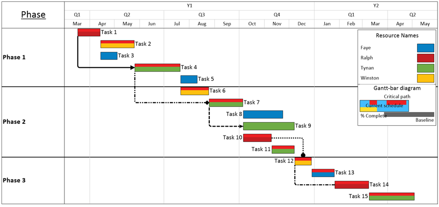
Project Critical Path in a Report | OnePager Pro
Display data point labels outside a pie chart in a paginated report ... Create a pie chart and display the data labels. Open the Properties pane. On the design surface, click on the pie itself to display the Category properties in the Properties pane. Expand the CustomAttributes node. A list of attributes for the pie chart is displayed. Set the PieLabelStyle property to Outside. Set the PieLineColor property to Black.

Elements of an Excel Chart | ExcelDemy.com
How to Show Percentage in Pie Chart in Excel? - GeeksforGeeks 29/06/2021 · It can be observed that the pie chart contains the value in the labels but our aim is to show the data labels in terms of percentage. Show percentage in a pie chart: The steps are as follows : Select the pie chart. Right-click on it. A pop-down menu will appear. Click on the Format Data Labels option. The Format Data Labels dialog box will appear.

Gantt chart - YouTube
How to Show Percentages in Stacked Column Chart in Excel? By default, the data labels are shown in the form of chart data Value (Image 1). But very often user needs to plot charts with actual data and show percentages/custom values on the chart instead of default data. For that we have an option "Value From Cells" in chart "Format Data Label" (Image 2) to select a custom range. Image 1 Image 2

Waterfall Chart in Excel - Easiest method to build.
How to Print Labels From Excel - Lifewire Choose Start Mail Merge > Labels . Choose the brand in the Label Vendors box and then choose the product number, which is listed on the label package. You can also select New Label if you want to enter custom label dimensions. Click OK when you are ready to proceed. Connect the Worksheet to the Labels
Fixing Your Excel Chart When the Multi-Level Category Label Option is Missing. - Excel Dashboard ...
Create Dynamic Chart Data Labels with Slicers - Excel Campus 09/02/2016 · Typically a chart will display data labels based on the underlying source data for the chart. In Excel 2013 a new feature called “Value from Cells” was introduced. This feature allows us to specify the a range that we want to use for the labels. Since our data labels will change between a currency ($) and percentage (%) formats, we need a ...
Post a Comment for "38 how to show labels in excel chart"